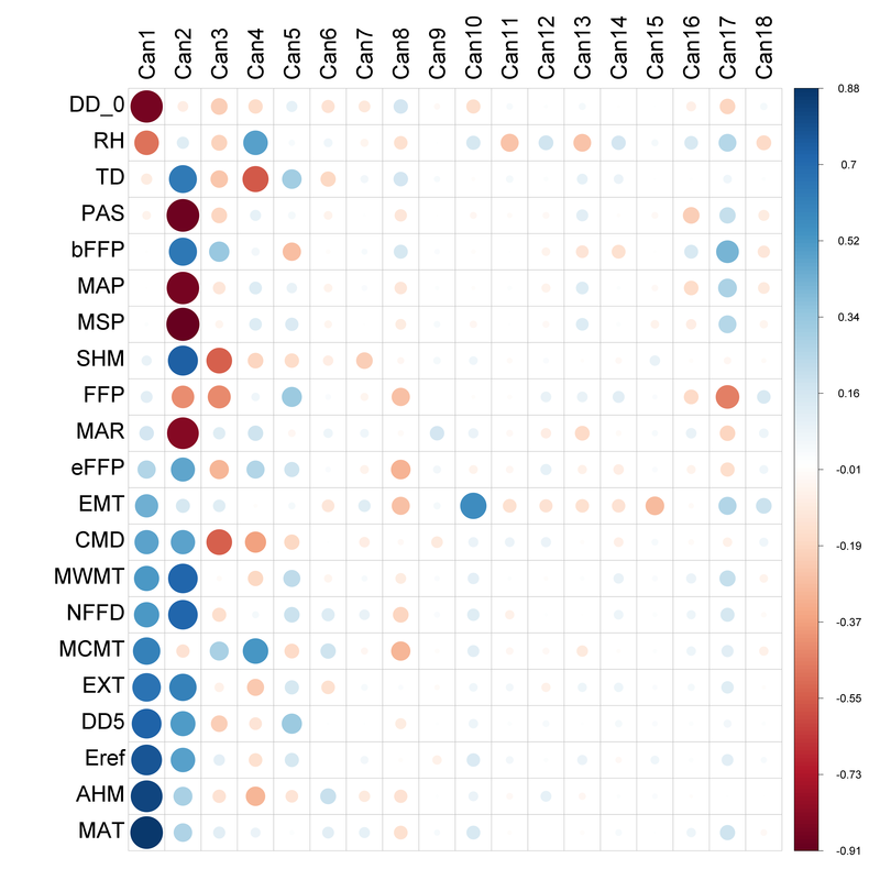
What are the climate variables that separate bioclimate zones?A Linear Discriminant Analysis (LDA) was conducted to compare the reference period 1961-1990 climate normals for twenty annual direct and derived climate variables. Variance explained in the first four principle components were 45.1%, 25.8%, 9.8% and 6.5%. Eigen values or loadings calculated by the LDA along for each climate variable are presented in Figure 7 with the first function sorted from largest to smallest.
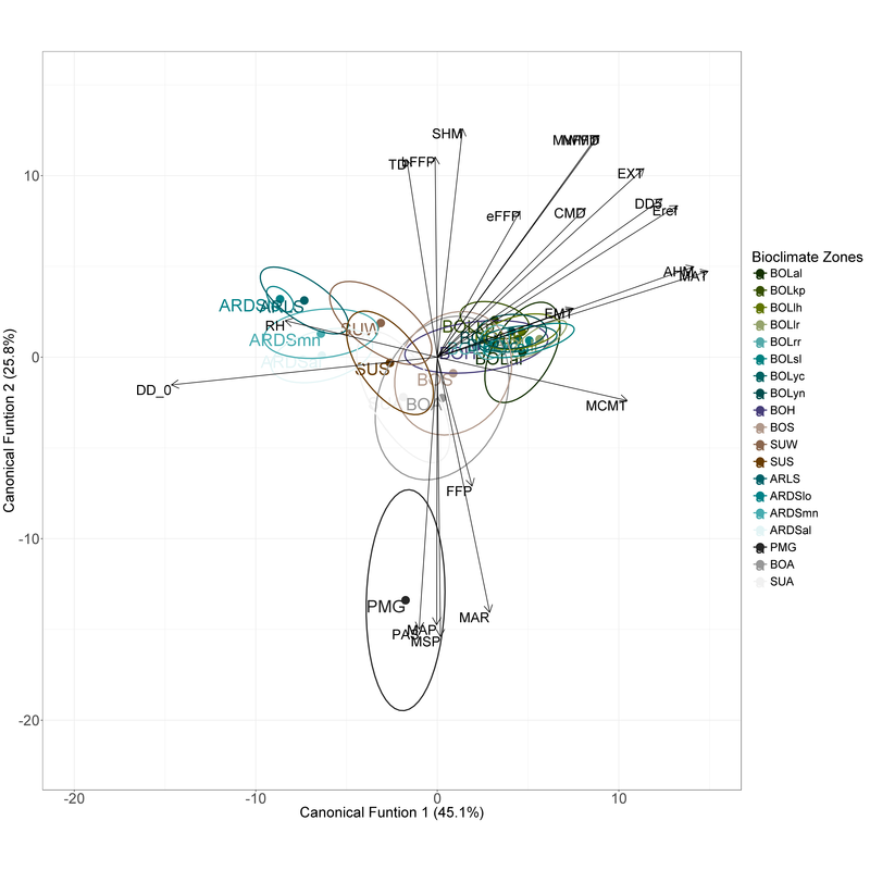
The ordination space for the LDA analysis for principle components 1 and 2 are shown in Figure 8. Results of the LDA show that bioclimate zones separate well in ordination space, meaning they can be distinguished using climate variables. The first principle component separates Arctic by DD<0 (positive) and Subarctic and Boreal regions by MAT and AHM (positive). Climate variables that separate Subarctic and Boreal regions are DD>5 and Eref which are representative of growing and drought potential, respectively. The second principle component
|
separated cold-wet pacific influenced regions by MSP, PAS, MAP and MAR. The second axis separated BOL subzones from BOH and Subarctic system by climate variables NFFD, MWMT and SHM which are related to frost free length, extremes between summer and winter wetness and summer heat, respectively.
These results suggest that there is a strong relationship between climatic variables (collectively the bioclimate envelope) and bioclimate subzones with 70.9% of the variance accounted for in the first two axis. My results suggest that there is reason to conclude that bioclimate envelope can be assessed and future bioclimate envelope space predicted using climate variables. The next section describes results of the random forest bioclimate envelope model of the 1961-90 reference period and prediction of how bioclimate subzone distribution changes with future climate periods.
|
|
|
|
Fig. 7 LDA reported Eigen values (or loadings) for each climate variable and climate variable characteristics for all subzones – sorted by the first discriminant function.
|
Fig. 8 Linear Discriminant Analysis Principle Components 1 and 2 showing mean value for loadings by bioclimate subzones (colours dots) and relationship with climate variables (Eigen Vectors).
|
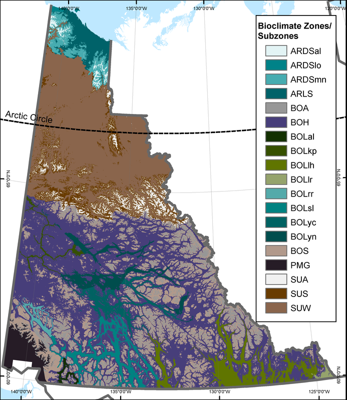
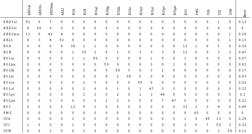
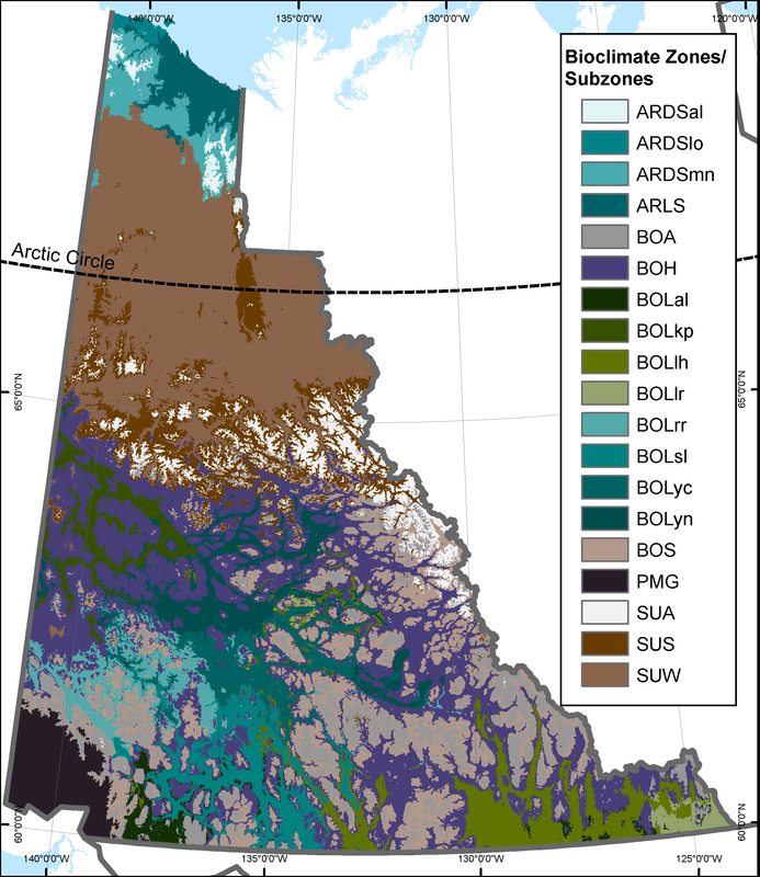
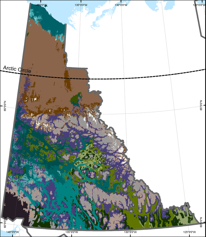
Will the distribution of climate zones change in the future?The resultant predicted bioclimate subzone map, modelled using random forest, is shown in Figure 9 along with the original bioclimate map from which the bioclimate envelope was derived, also using random forest. The confusion matrix reported by the random forest model (over all trees) is shown in Table 3. Overall classification accuracy using Cohan’s Kappa is 81%. Although the LDA shows that bioclimate regions are well predicted by climate variables and the spatial distribution and overall classification accuracy is high, inspection of the confusion matrix shows there is a fair amount of error in classification accuracy associated with the Boreal High (BOH) subzone. BOH is often confused with the subzone BOS which sits just above BOH. Likely this is due to the large geographic range of BOH latitudinally (Figure 9). Although there is some mixing across subzones that are elevational near-neighbors, the magnitude of shift in climate variables between periods is greater than the classification error.
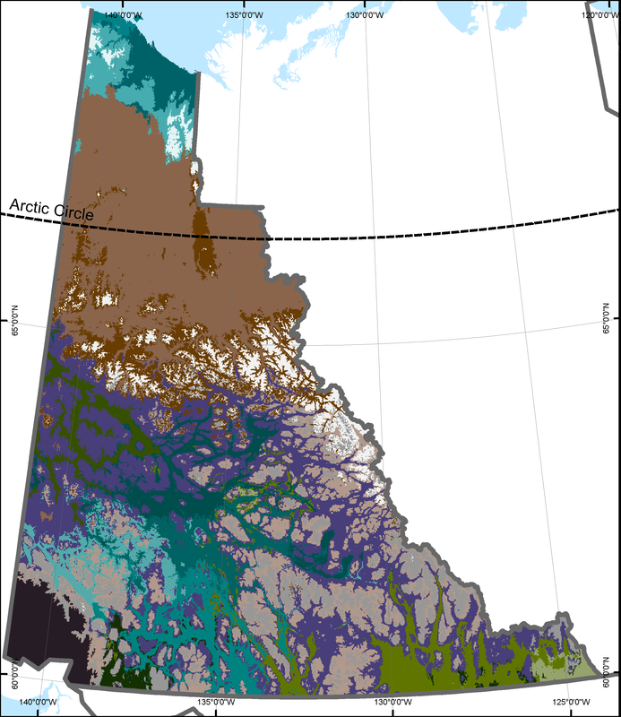
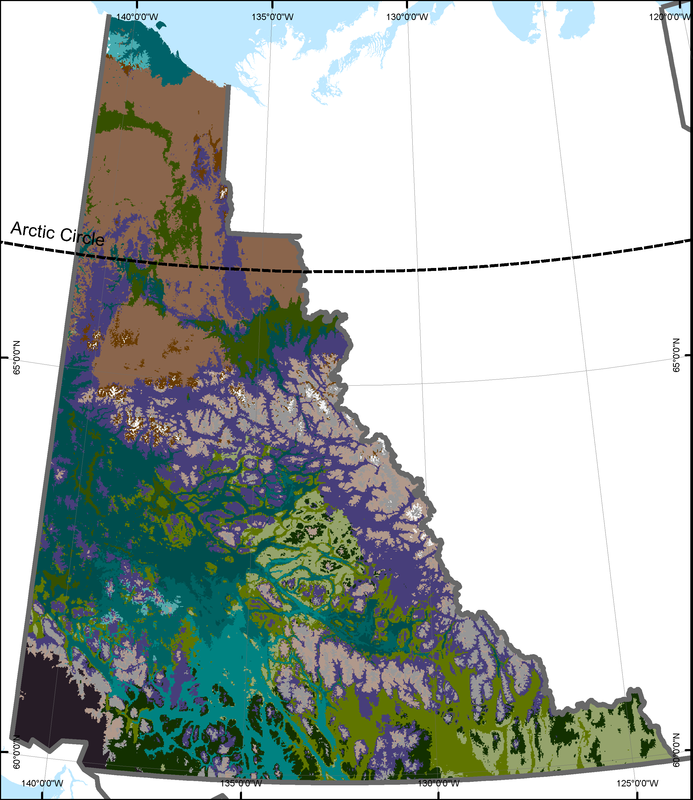
I applied the bioclimate envelopes to two future climate periods. Figure 10 shows the predicted bioclimate envelopes for 1991-2016 and 2025 climate periods. This climate change time series shows two patterns. Firstly, lower elevation Boreal Low subzones often stayed within the Boreal Low zone designation but often shifted to a BOL subzone that occurs more commonly in
|
southern latitudes. Secondly, the BOH subzone, which often
occurs elevationally above BOL, shifted to a BOL subzone bioclimate. In general, higher elevation subzones shifted to a BOL subzone typically associated with lower elevations. This trend can be seen clearly comparing the 1961-90 and 1991-2016 predicted bioclimate maps. Figure 11 shows a bar chart of total area (km2) each bioclimate zone occupies in the reference period (1961-1990) and its area (km2) attributed to membership in the same or another subzone in the 1991-2016 and 2025 periods. As expected BOL subzones are “replaced” by BOL subzones from southern Yukon. Due to a combination of climate and topography SUW and BOH comprise the significant portion of the Yukon’s forested regions. SUW or subarctic woodland is a high latitude subzone that covers a broad extent. BOH or Boreal High is also found in higher latitudes but also occurs at mid-elevation at southern latitudes. These results show that BOH has already experienced dramatic shifts in its climate characteristics – with nearly 50% being characteristic of lower elevation and latitudes Boreal Low climatic conditions. SUW is relatively “stable” but is expected to shift as well in the very near future.
|
|
|
Figure 9 Original (9a) and predicted bioclimate envelope (9b) for the 1961-90 reference period climate variables using RandomForest and 60 points randomly place in each bioclimate subzone.
Table 3 Random Forest confusion matrix showing degree of agreement between and amongst actual (columns) and predicted (rows) bioclimate zones. Cohen’s Kappa (based on all trees) = 0.81.
|
|
|
Fig. 10 a,b,c Projected Bioclimate Envelopes for 1961-1990 (10a), 1991-2016 period (10b) and 2025 (10c).
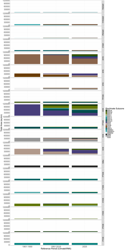
Fig. 11 Bar chart of total area (km2) each bioclimate zone occupies in the reference period (1961-1990) and its area (km2) with membership in a subzone in the 1991-2016 period and 2025 periods.
