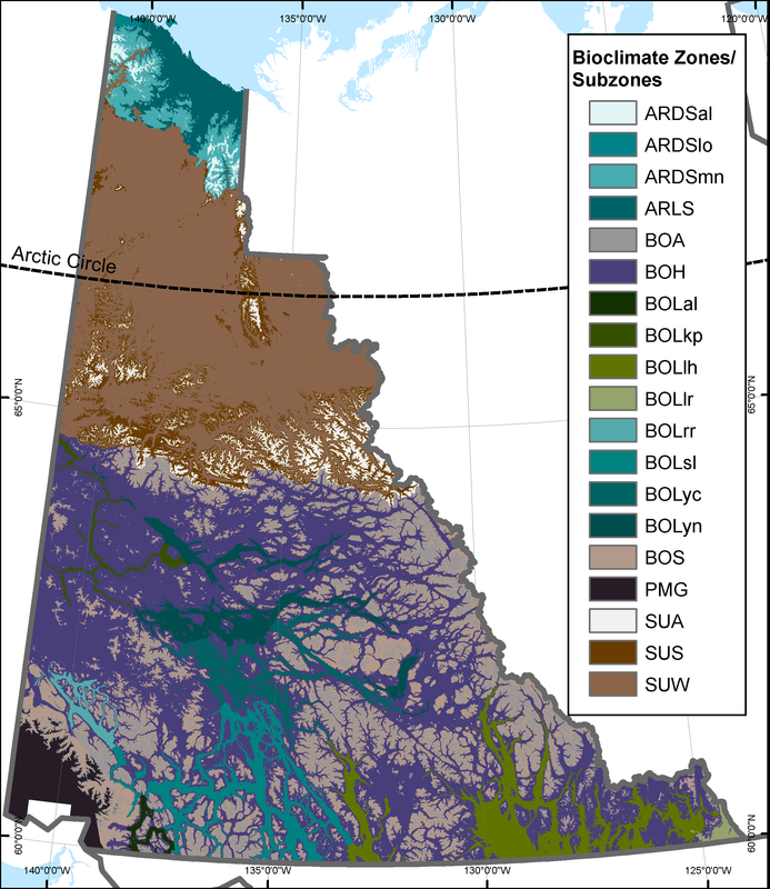
Data AssemblyI used bioclimate map of Yukon (Department of Environment 2016) to develop a bioclimate envelope for the reference period 1961-1990. Figure 1 shows bioclimate zones and subzones in Yukon used in this study. The reference period served as a base for predicting the distribution of bioclimate subzones for a later 1991-2016 period and a 2025 future period. The Yukon bioclimate map is a delineation of vegetation that reflects a zonal condition and is characterized by long-term climatic conditions that gives rise to a plant community that reflects the regional climate. In the bioclimate system the zone describes a broader climatic continental delineation of climatic zones. Subzones divide zones into finer spatial units that represent climatic differences within zones that give rise to differentiation in zonal plant communities. Currently only Boreal Low zones are subdivided into subzones. For the purposes of this analysis, zones that are not subdivided into subzones are treated as their own subzone.
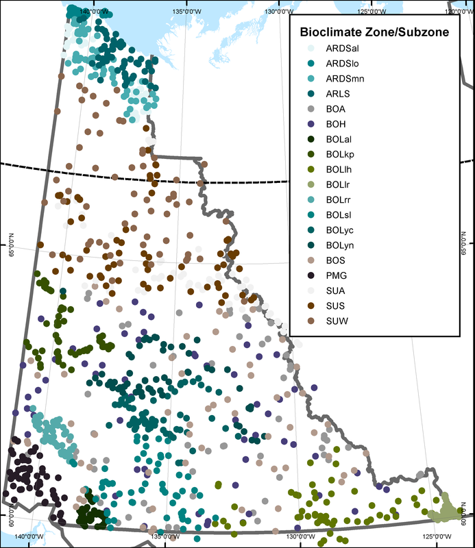
I randomly assigned 60 points to each subzone in the bioclimate map. The population of random plots is considered representative of the broader population of bioclimate subzones. The distribution of random points in the study area is shown in Figure 2. Climate variables at the resolution of 4 x 4 km were generated for all random points used the downscaling algorithms developed for ClimateWNA (Wang et al 2012) for the reference normal period 1961-1990, 1991-2016 and one future period 2025. The future climate data was generated based on the general circulation models MIROC5-RCP4.5 from IPCC Fifth Assessment Report (IPCC 2014). Annual climate data available in ClimateWNA (Wang et al 2012) for years 1991 to 2016 were averaged across annual climate variables. Although the total is 25 years I considered this an adequate climate period for analysis. Twenty annual direct and derived climate variables, used for reference and future climate periods, are listed in Table 1.
The elevation grid used to generate ClimateWNA climate variables was assembled for the entire study area from Advanced Spaceborne Thermal Emission and Reflection Radiometer Global Digital Elevation Model Version 2 (ASTER Global Digital Elevation Model v2). The ASTER GDEM v2 was projected from its native geographic projection to a Yukon Albers
|
projection with a pixel resolution of 25 meters. The DEM was resampled to
1 km resolution using the aggregate method in ArcInfo GIS 10.5 Spatial Analyst tool to increase processing speed of the model. AnalysisI used Linear Discriminant Analysis to describe a linear combination of climate variables that best describe how bioclimate zones are distinct from each other and a machine learning technique, RandomForest (Liaw and Wiener 2002) to model the bioclimate envelope based on the reference normal period 1961-90. The RandomForest model, developed from the reference period climate data, was applied to a 1km ASTER DEM with climate variables “tied” to the centre of each DEM pixel. This created a surface of the predicted distribution of bioclimate zones for other periods. Climate variables were assessed for univariate homogeneity of variance using Levene’s test of homogeneity of variance (Levene 1960). Box's M-test (F-ratio test) test equality of variance-covariance matrices. All statistical analysis was done using R 3.4.1 (R Core Team 2013).
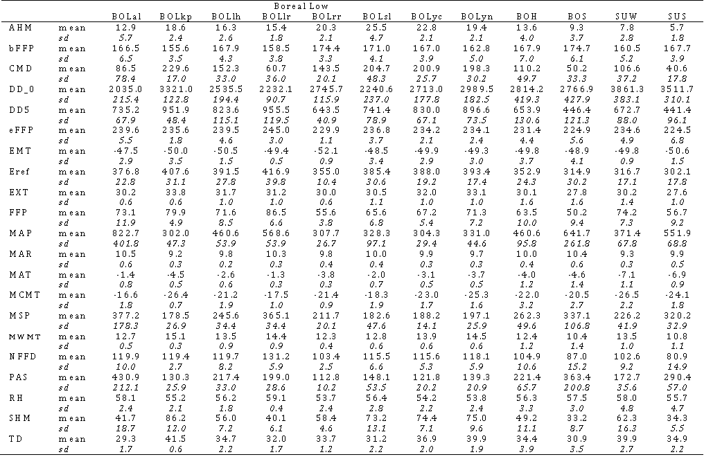
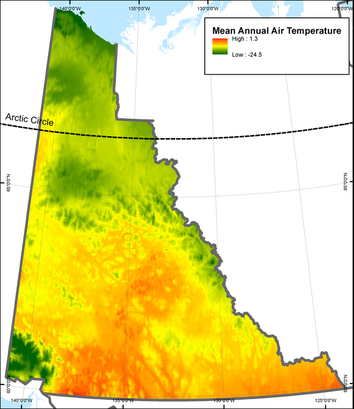
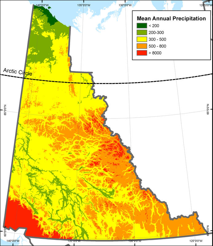
Data ExplorationDescriptive statistics using boxplots are presented in this section as a preliminary analysis of trends and patterns of climate variables associated with bioclimate subzones as determined by randomly selected points. A boxplot shows the distribution of data using the minimum, first quartile, median, third quartile and maximum. Figures 3 and 4 show the boxplot of reference period climate variables MAT and MAP by bioclimate subzone. Bioclimate subzones vary in their distribution for MAT and MAP demonstrating that subzones do vary climatically. Other climate variables examined, but not presented here, also show variability with climate. Figure 5 and 6 shows the spatial distribution of reference period climate variables MAT and MAP throughout Yukon. Table 2 shows mean values and standard deviations for climate variables associated with random points for the reference period (1961-1991) by subzone.
|
|
|
|
Fig. 1 Distribution of bioclimate subzones used for discriminant analysis and bioclimate envelop modeling of zones in Yukon
|
Fig. 2 Distribution of random points (~60 per subzone) used to build bioclimate envelope model for Yukon subzones.
|
Table 1 Climate variables (annual direct and derived) used for discriminant analysis and bioclimate envelop modeling of bioclimate subzones in Yukon.
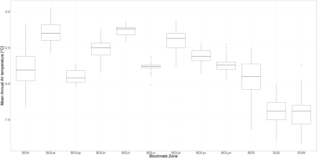
Fig 3 Boxplot comparing the relationship between reference period (1961-1990) climate variable Mean Annual Air Temperature (C°) by bioclimate subzone.
|
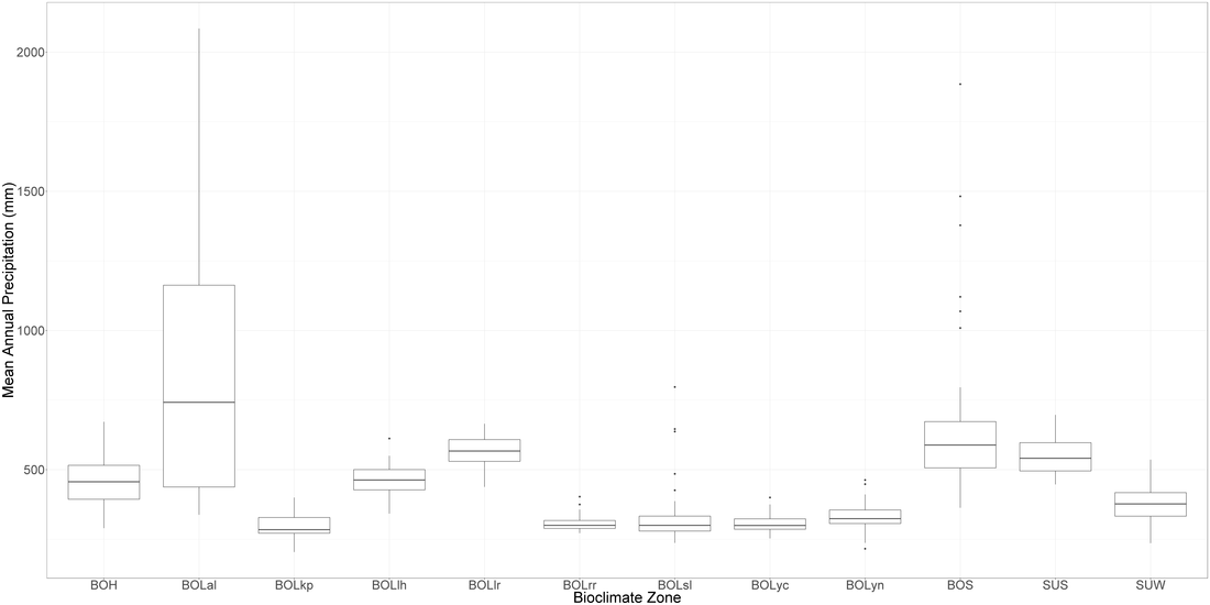
Fig. 4 Boxplot comparing the relationship between reference period (1961-1990) climate variable Mean Annual Precipitation (mm) by bioclimate subzone.
|
|
|
|
Fig. 5 Map of Mean Annual Air Temperature (C°) for Yukon derived from the 1961-90 Reference Period for climate variables generated by ClimateWNA, resolution is 1km2 pixel.
|
Fig. 6 Map of Mean Annual Precipitation (mm) for Yukon derived from the 1961-90 Reference Period for climate variables generated by ClimateWNA, resolution is 1km2 pixel.
|
Table 2 Mean climate normal (1961-1991) and standard deviations for bioclimate subzones used for zone analysis based on 60 randomly selected points per subzone (Arctic, Pacific and Alpine zones are not shown).